Asian option pricing - A quasi-Monte Carlo approach

Introduction

In this project, I am using Monte Carlo simulation approach to price a hypothetical asian option in a hypothetical environment. My objective is to compare performance of quasi-Monte Carlo methods (using Sobol and Halton sequences) with ordinary Monte Carlo simulation.

Performance Comparison

Performance comparison is done in terms of the largest sample size, by which a method can reach (required) small enough precision (which is proportionate to confidence interval length of the estimation). We will assume that required threshold for confidence interval length is 0.5 dollar.

Quasi-Monte Carlo Method

Quasi-Monte Carlo method for simulation is used in order to get required precision with smaller sample sizes. This approach uses low-descrepancy sequences for simulation instead of psuedorandom numbers in the ordinary Monte Carlo methods.

Asian option

Asian options is a path-dependant option in which the payoff depends on average price of an underlying asset during the option period. The type option we price here is average-price asian call option which has the payoff:

\[payoff = max\{average(price) - X\}\]

Where is X is the exercise price of the option.

Underlying asset process

Price of the underlying asset is assumed to follow the stochastic process of geometric brownian motion which means:

\[S(t + \Delta t) = S(t)e^{(r - \frac{\sigma ^2}{2})\Delta t + \sigma \epsilon \sqrt{\Delta t}}\]

!pip install chaospy

import numpy as np
import chaospy as ch
from scipy import stats
import matplotlib.pyplot as plt

%matplotlib inline

Defining some helper functions

def payoff_calc(price_array, X):
    """
    This function calculates future payoff of the asian option based on arithmetic average of the price path
    
    INPUT:
        price_array (numpy.ndarray): A one-dimensional array of stock final prices
        X (float): Exercise price of the option
    
    OUTPUT:
        (numpy.ndarray): A one dimensional array of payoffs for different prices
    """
    
    payoff = np.maximum(0, np.mean(price_array) - X)
    return payoff

def pv_calc(FV, r, T):
    """
    Calculates present value of an amount of money in future.
    
    INPUT:
        FV (float): Future value of money
        r (float): Risk neutral interest rate
        T (float): Period of time
    
    OUTPUT:
        (float): Present value of FV
    """
    
    return FV * np.exp(-r * T)

def CI_calc(s_array):
    """
    Calculates 95% confidence interval for the estimation of expected value of a random variable, given a sample.
    
    INPUT:
        s_array (Numpy.ndarray): A one-dimensional array of the sample
    
    OUTPUT:
        (Numpy.ndarray): with shape==(1,2) which has lower and upper bound of the confidence interval
    """
    
    X_bar = np.mean(s_array)
    Upper_b = X_bar + (np.sqrt(np.var(s_array)) * stats.norm.ppf(0.975)) / np.sqrt(len(s_array))
    Lower_b = X_bar - (np.sqrt(np.var(s_array)) * stats.norm.ppf(0.975)) / np.sqrt(len(s_array))
    return np.array([Lower_b, Upper_b])

def sobol_generator(m, n):
    """
    Generates m samples (each for one path) each having n numbers in Sobol sequence.
    
    INPUT:
        m (int): number of samples
        n (int): number of Sobol sequence numbers in each sample
        
    OUTPUT:
        (numpy.ndarray): A two-dimensional array of Sobol sequence numbers for conducting QMC simulation
    """
    sob_array = np.empty((0, n))
    for i in range(m // 39 + 1):
        sob = ch.create_sobol_samples(n, 39, i)
        sob_array = np.append(sob_array, sob, axis=0)
    return sob_array

def halton_generator(m, n):
    """
    Generates m samples each having n numbers in Halton sequence.
    
    INPUT:
        m (int): The order of Halton sequence. Defines the number of samples
        n (int): Dimension of each sequence.Defines the number of Halton sequence numbers in each sample.
        
    OUTPUT:
        (numpy.ndarray): A two-dimensional array of Sobol sequence numbers for conducting QMC simulation
    """
    hal_seq = ch.create_halton_samples(m, n)
    return hal_seq

def sobol_seq_sim(no_of_paths, n_steps, S_0, T, r, sigma, x_price):
    """
    Conducts QMC simulation using Sobol sequence.
    
    INPUT:
        no_of_paths (int): Number of samples in simulation
        n_steps (int): Number of price step we aim to simulate in each path
        S_0 (float): Underlying asset price at time zero
        T (float): Time period of option contract
        r (float): Risk-netural interest rate
        sigma (float): Volatility in the environment
        x_price (float): Exercise price of the option
        
    OUTPUT:
        (Numpy.ndarray): A one-dimensional array of present value of simulated payoffs
    """
    dt = T / n_steps
    present_payoffs = np.zeros(no_of_paths)
    epsilon_s = stats.norm.ppf(sobol_generator(no_of_paths, n_steps))
    
    for k in range(no_of_paths):
        price_steps = np.zeros(n_steps)
        price_steps[0] = S_0
        for i in range(1, n_steps):
            price_steps[i] = price_steps[i-1] * np.exp((r - sigma ** 2 / 2) * dt + sigma * epsilon_s[k, i] * np.sqrt(dt))
        present_payoffs[k] = pv_calc(payoff_calc(price_steps, x_price), r, T)
    return present_payoffs

def halton_seq_sim(no_of_paths, n_steps, S_0, T, r, sigma, x_price):
    """
    Conducts QMC simulation using Halton sequence.
    
    INPUT:
        no_of_paths (int): Number of samples in simulation
        n_steps (int): Number of price step we aim to simulate in each path
        S_0 (float): Underlying asset price at time zero
        T (float): Time period of option contract
        r (float): Risk-netural interest rate
        sigma (float): Volatility in the environment
        x_price (float): Exercise price of the option
        
    OUTPUT:
        (Numpy.ndarray): A one-dimensional array of present value of simulated payoffs
    """
    dt = T / n_steps
    present_payoffs = np.zeros(no_of_paths)
    epsilon_h = stats.norm.ppf(halton_generator(no_of_paths, n_steps))
    
    for k in range(no_of_paths):
        price_steps = np.zeros(n_steps)
        price_steps[0] = S_0
        for i in range(1, n_steps):
            price_steps[i] = price_steps[i-1] * np.exp((r - sigma ** 2 / 2) * dt + sigma * epsilon_h[i, k] * np.sqrt(dt))
        present_payoffs[k] = pv_calc(payoff_calc(price_steps, x_price), r, T)
    return(present_payoffs)

def ordinary_mc_sim(no_of_paths, n_steps, S_0, T, r, sigma, x_price):
    """
    Conducts MC simulation,
    
    INPUT:
        no_of_paths (int): Number of samples in simulation
        n_steps (int): Number of price step we aim to simulate in each path
        S_0 (float): Underlying asset price at time zero
        T (float): Time period of option contract
        r (float): Risk-netural interest rate
        sigma (float): Volatility in the environment
        x_price (float): Exercise price of the option
        
    OUTPUT:
        (Numpy.ndarray): A one-dimensional array of present value of simulated payoffs
    """
    dt = T / n_steps
    present_payoffs = np.zeros(no_of_paths)
    epsilon = np.random.normal(0, 1, (no_of_paths, n_steps))
    
    for k in range(no_of_paths):
        price_steps = np.zeros(n_steps)
        price_steps[0] = S_0
        for i in range(1, n_steps):
            price_steps[i] = price_steps[i-1] * np.exp((r - sigma ** 2 / 2) * dt + sigma * epsilon[k, i] * np.sqrt(dt))
        present_payoffs[k] = pv_calc(payoff_calc(price_steps, x_price), r, T)
    return(present_payoffs)

def sim_iterator(max_sample, n_steps, S_0, T, r, sigma, x_price, *,method):
    """
    Iterates simulation with different sample sizes (form 10 to a maximum size with steps of 10)
    and records estimated price as well as confidence interval of the estimation
    
    INPUT:
        max_sample (int): Maximum sample size for the iteration of simulations
        n_steps (int): Number of price step we aim to simulate in each path
        S_0 (float): Underlying asset price at time zero
        T (float): Time period of option contract
        r (float): Risk-netural interest rate
        sigma (float): Volatility in the environment
        x_price (float): Exercise price of the option
        method (string): 'sobol', 'halton' or 'ordinary'
    
    OUTPUT:
        (numpy.ndarray): confidence intervals of the simulations
        (numpy.ndarray): price estimations of the simulations
    """
    
    assert(method in ['sobol', 'halton', 'ordinary'])
    
    mean_pv_payoffs = np.zeros(int(np.ceil(max_sample / 10)))
    confidence_intervals = np.array([None, None])
    
    if method == 'sobol':
        for n_sample in range(10, max_sample + 1, 10):
            present_payoffs = sobol_seq_sim(n_sample, n_steps, S_0, T, r, sigma, x_price)
            mean_pv_payoffs[int(n_sample/10 - 1)] = np.mean(present_payoffs)
            confidence_intervals = np.row_stack((confidence_intervals, CI_calc(present_payoffs)))
    
    elif method == 'halton':
        for n_sample in range(10, max_sample + 1, 10):
            present_payoffs = halton_seq_sim(n_sample, n_steps, S_0, T, r, sigma, x_price)
            mean_pv_payoffs[int(n_sample/10 - 1)] = np.mean(present_payoffs)
            confidence_intervals = np.row_stack((confidence_intervals, CI_calc(present_payoffs)))
    
    elif method == 'ordinary':
        for n_sample in range(10, max_sample + 1, 10):
            present_payoffs = ordinary_mc_sim(n_sample, n_steps, S_0, T, r, sigma, x_price)
            mean_pv_payoffs[int(n_sample/10 - 1)] = np.mean(present_payoffs)
            confidence_intervals = np.row_stack((confidence_intervals, CI_calc(present_payoffs)))

    
    return confidence_intervals, mean_pv_payoffs

def CI_length_calc(CI):
    """
    Calculates length of a confidence interval.
    
    INPUT:
        CI (numpy.ndarray): Confidence intervals
    
    OUTPUT:
        (numpy.ndarray): lengths of the confidence intervals
    """
    
    return CI[1:, 1] - CI[1:, 0]

def threshold_finder(CI, tol):
    """
    In an array of confidence intervals in the order of descending lengths,
    returns the index of fist interval shorter than a threshold.
    
    INPUT:
        CI (numpy.ndarray): Confidence intervals
        tol (float): length threshold
    
    OUTPUT:
        (int): the index of fist interval shorter than 'tol'.
    """
    
    CI_length = CI_length_calc(CI)
    for i, length in enumerate(CI_length):
        if length <= tol:
            return i
    else:
        return None

Conducting the simulations

r = 0.1
sigma = 0.2
T = 2
n_steps = 20
dt = T / n_steps
S_0 = 50
x_price = 40

max_sample = 7000


sobol_CIs, sobol_price_esitmates = sim_iterator(max_sample, n_steps, S_0, T, r, sigma, x_price, method='sobol')
halton_CIs, halton_price_esitmates = sim_iterator(max_sample, n_steps, S_0, T, r, sigma, x_price, method='halton')
ordinaryMC_CIs, ordinaryMC_price_esitmates = sim_iterator(max_sample, n_steps, S_0, T, r, sigma, x_price, method='ordinary')

print("Price estimated at largest sample size with Sobol sequence:", str(sobol_price_esitmates[-1]))
print("CI length at largest sample size with Sobol sequence:", str(sobol_CIs[-1,1] - sobol_CIs[-1,0]))

print("Price estimated at largest sample size with Halton sequence:", str(halton_price_esitmates[-1]))
print("CI length at largest sample size with Halton sequence:", str(halton_CIs[-1,1] - halton_CIs[-1,0]))

print("Price estimated at largest sample size with ordinary MC:", str(ordinaryMC_price_esitmates[-1]))
print("CI length at largest sample size with ordinary MC:", str(ordinaryMC_CIs[-1,1] - ordinaryMC_CIs[-1,0]))

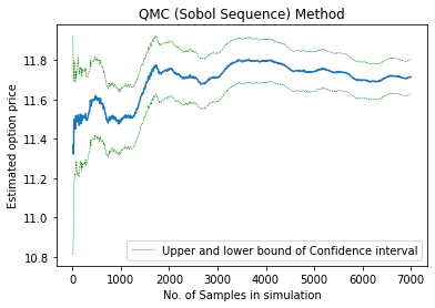
Price estimated at largest sample size with Sobol sequence: 11.715011344960544
CI length at largest sample size with Sobol sequence: 0.17423024315435853
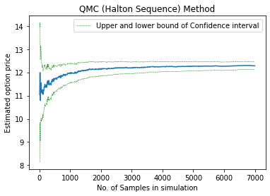
Price estimated at largest sample size with Halton sequence: 12.280725716144751
CI length at largest sample size with Halton sequence: 0.3330768226385423
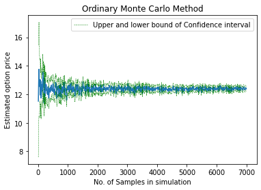
Price estimated at largest sample size with ordinary MC: 12.388931350290722
CI length at largest sample size with ordinary MC: 0.33597514567397013

Ploting the results

#Ploting ordinary Monte Carlo method
x_axis1 = range(10, max_sample + 1, 10)
plt.plot(x_axis1, ordinaryMC_price_esitmates)
plt.plot(x_axis1, ordinaryMC_CIs[1:, 0], 'g--', lw=0.5, label='Upper and lower bound of Confidence interval')
plt.plot(x_axis1, ordinaryMC_CIs[1:, 1], 'g--', lw=0.5)
plt.xlabel("No. of Samples in simulation")
plt.ylabel("Estimated option price")
plt.title("Ordinary Monte Carlo Method")
plt.legend()
plt.show()

#Ploting quasi-Monte Carlo method using Sobol sequence

plt.plot(x_axis1, sobol_price_esitmates)
plt.plot(x_axis1, sobol_CIs[1:, 0], 'g--', lw=0.5, label='Upper and lower bound of Confidence interval')
plt.plot(x_axis1, sobol_CIs[1:, 1], 'g--', lw=0.5)
plt.xlabel("No. of Samples in simulation")
plt.ylabel("Estimated option price")
plt.title("QMC (Sobol Sequence) Method")
plt.legend()
plt.show()

#Ploting quasi-Monte Carlo method using Halton sequence

plt.plot(x_axis1, halton_price_esitmates)
plt.plot(x_axis1, halton_CIs[1:, 0], 'g--', lw=0.5, label='Upper and lower bound of Confidence interval')
plt.plot(x_axis1, halton_CIs[1:, 1], 'g--', lw=0.5)
plt.xlabel("No. of Samples in simulation")
plt.ylabel("Estimated option price")
plt.title("QMC (Halton Sequence) Method")
plt.legend()
plt.show()

Comparison and Conclusion

tol = 0.5
sobol_threshold = threshold_finder(sobol_CIs, tol)
halton_threshold = threshold_finder(halton_CIs, tol)
mc_threshold = threshold_finder(ordinaryMC_CIs, tol)

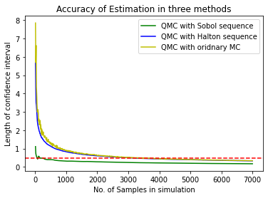
print("Largest sample size by which ordinary MC can reach CI shorter than 0.5 dollor is:", str(mc_threshold*10))
print("Largest sample size by which QMC using Sobol sequence can reach CI shorter than 0.5 dollor is:", str(sobol_threshold*10))
print("Largest sample size by which QMC using Halton sequence can reach CI shorter than 0.5 dollor is:", str(halton_threshold*10))

Largest sample size by which ordinary MC can reach CI shorter than 0.5 dollor is: 3090
Largest sample size by which QMC using Sobol sequence can reach CI shorter than 0.5 dollor is: 50
Largest sample size by which QMC using Halton sequence can reach CI shorter than 0.5 dollor is: 3000

sobol_CI_lengths = CI_length_calc(sobol_CIs)
halton_CI_lengths = CI_length_calc(halton_CIs)
ordinary_CI_lengths = CI_length_calc(ordinaryMC_CIs)

plt.plot(x_axis1, sobol_CI_lengths, 'g', label="QMC with Sobol sequence")
plt.plot(x_axis1, halton_CI_lengths, 'b', label="QMC with Halton sequence")
plt.plot(x_axis1, ordinary_CI_lengths, 'y', label="QMC with oridnary MC")

plt.axhline(tol, ls='--', c='r')
plt.xlabel("No. of Samples in simulation")
plt.ylabel("Length of confidence interval")
plt.title("Accuracy of Estimation in three methods")
plt.legend()
plt.show()

Simulation Method	Estimated Price at largest sample	Convergence sample size	CI length at largest sample
Ordinary MC	$12.39	3090	0.34
Sobol sequence	$11.72	50	0.17
Halton Sequence	$12.28	3000	0.33