Performance of LR, Wald and score tests with respect to sample size
In this blog post I compare how performance of Likelihood ratio (LR), Wald and score test change with respect to sample size. GLM set chosen for this purpose is a binomial response variable with a single independent variable (X). We use the typical logit link function for modeling.
LR Test
#Examining Deviance test
set.seed(1366)
NREP = 500
sample_n = 100  #This variable shows number of steps for sample size. each steps will increase by 5
beta_A = c(0.1,0.2,0) #null hypothesis is true
beta_B = c(0.1, 0.2,-0.1)  #null hypothesis is false

Wrong_Dec_matrix = matrix(0,sample_n,5)
colnames(Wrong_Dec_matrix) <- c("Sample Size","Wrong_Rejections", "Wrong_acceptance", "Wrong_Decision", "Wrong_Decisions_Ratio")

for (k in 1:sample_n){
  sample_size = k * 5
  Null_Rej_DevianceT = matrix(0, NREP, 2)
  for (i in 1:NREP){
    x1 <- runif(sample_size,min = -2, max=2)
    x2 <- rnorm(sample_size, 0, 2)
    y_A <- rbinom(sample_size, size = 20, prob = 1/(1+exp(-(cbind(1,x1,x2) %*% beta_A))))
    y_B <- rbinom(sample_size, size = 20, prob = 1/(1+exp(-(cbind(1,x1,x2) %*% beta_B))))

    Full_model_A <- glm(cbind(y_A , 20-y_A) ~ cbind(x1,x2), family = binomial())
    Red_model_A <- glm(cbind(y_A , 20-y_A) ~ x1, family = binomial())

    Full_model_B <- glm(cbind(y_B , 20-y_B) ~ cbind(x1,x2), family = binomial())
    Red_model_B <- glm(cbind(y_B , 20-y_B) ~ x1, family = binomial())

    Null_Rej_DevianceT[i,1] <- as.numeric(deviance(Red_model_A) - deviance(Full_model_A) > qchisq(0.95, 1))

    Null_Rej_DevianceT[i,2] <- as.numeric((deviance(Red_model_B) - deviance(Full_model_B)) > qchisq(0.95, 1))
  }
  Wrong_Dec_matrix[k,1] = sample_size
  Wrong_Dec_matrix[k,2] = sum(Null_Rej_DevianceT[,1])
  Wrong_Dec_matrix[k,3] = NREP - sum(Null_Rej_DevianceT[,2])
  Wrong_Dec_matrix[k,4] = Wrong_Dec_matrix[k,2] + Wrong_Dec_matrix[k,3]
  Wrong_Dec_matrix[k,5] = Wrong_Dec_matrix[k,4] / NREP
}

print(head(Wrong_Dec_matrix,10))
##       Sample Size Wrong_Rejections Wrong_acceptance Wrong_Decision Wrong_Decisions_Ratio
##  [1,]           5               34              431            465                 0.930
##  [2,]          10               26              378            404                 0.808
##  [3,]          15               25              339            364                 0.728
##  [4,]          20               26              282            308                 0.616
##  [5,]          25               24              243            267                 0.534
##  [6,]          30               23              196            219                 0.438
##  [7,]          35               35              148            183                 0.366
##  [8,]          40               19              114            133                 0.266
##  [9,]          45               29               84            113                 0.226
## [10,] 50 16 74 90 0.180print(tail(Wrong_Dec_matrix,10))
##        Sample Size Wrong_Rejections Wrong_acceptance Wrong_Decision Wrong_Decisions_Ratio
##  [91,]         455               18                0             18                 0.036
##  [92,]         460               21                0             21                 0.042
##  [93,]         465               20                0             20                 0.040
##  [94,]         470               26                0             26                 0.052
##  [95,]         475               20                0             20                 0.040
##  [96,]         480               29                0             29                 0.058
##  [97,]         485               19                0             19                 0.038
##  [98,]         490               21                0             21                 0.042
##  [99,]         495               27                0             27                 0.054
## [100,]         500               20                0             20                 0.040
In the following plot, we can see how accuracy of LR test increases with regard to sample size:
plot(Wrong_Dec_matrix[,1], Wrong_Dec_matrix[,5], type = "l", lty=1, lwd=2, xlab = "Sample Size", ylab = "Wrong decision ratio", main = "Accuracy of LR test in different sample sizes")
lines(Wrong_Dec_matrix[,1], Wrong_Dec_matrix[,2]/NREP, col="red",lty=2)
lines(Wrong_Dec_matrix[,1], Wrong_Dec_matrix[,3]/NREP, col="blue",lty=3)
legend("topright",c("Wrong decision ratio","Wrong rejection ratio","Wrong acceptance ratio"),lty=1:3,lwd=c(2,1,1),col = c("black","red","blue"))
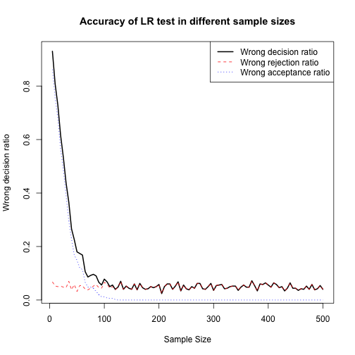
As we can see in the plot above when sample size increases, accuracy for LR test also increases and converges to its best amount (i.e. about %5 of wrong decision). We can see that for sample sizes greater than 200 (approximately) we do not see considerable improvement in accuracy. Also we should note that the factor that improves the accuracy of decisions is decrease in the rate of wrong acceptance ratio when the reduced model is not adequate but we do not reject it in favor of full model. Wrong rejection of reduced model does not get significantly better by increaseing sample size.
Wald and Score Test
We can show Wald and score statistics are the same for binomial model. So in the following chunk, I am implementing these two tests at the same time.
Wrong_Dec_matrix2 = matrix(0,sample_n,5)
colnames(Wrong_Dec_matrix2) <- c("Sample Size","Wrong_Rejections", "Wrong_acceptance", "Wrong_Decision", "Wrong_Decisions_Ratio")

for (k in 1:sample_n){
  sample_size = k * 5
  Null_Rej_Wald = matrix(0, NREP, 2)
  for (i in 1:NREP){
    x1 <- runif(sample_size,min = -2, max=2)
    x2 <- rnorm(sample_size, 0, 2)
    y_A <- rbinom(sample_size, size = 20, prob = 1/(1+exp(-(cbind(1,x1,x2) %*% beta_A))))
    y_B <- rbinom(sample_size, size = 20, prob = 1/(1+exp(-(cbind(1,x1,x2) %*% beta_B))))

    Full_model_A <- glm(cbind(y_A , 20-y_A) ~ cbind(x1,x2), family = binomial())
    #Red_model_A <- glm(cbind(y_A , 20-y_A) ~ x1, family = binomial())

    Full_model_B <- glm(cbind(y_B , 20-y_B) ~ cbind(x1,x2), family = binomial())
    #Red_model_B <- glm(cbind(y_B , 20-y_B) ~ x1, family = binomial())

    Null_Rej_Wald[i,1] <- as.numeric(abs(Full_model_A$coefficients[3]/sqrt(summary(Full_model_A)$cov.unscaled[3,3])) > qnorm(0.975))

    Null_Rej_Wald[i,2] <- as.numeric(abs(Full_model_B$coefficients[3]/sqrt(summary(Full_model_B)$cov.unscaled[3,3])) > qnorm(0.975))
  }
  Wrong_Dec_matrix2[k,1] = sample_size
  Wrong_Dec_matrix2[k,2] = sum(Null_Rej_Wald[,1])
  Wrong_Dec_matrix2[k,3] = NREP - sum(Null_Rej_Wald[,2])
  Wrong_Dec_matrix2[k,4] = Wrong_Dec_matrix2[k,2] + Wrong_Dec_matrix2[k,3]
  Wrong_Dec_matrix2[k,5] = Wrong_Dec_matrix2[k,4] / NREP
}
print(head(Wrong_Dec_matrix2,10))
##       Sample Size Wrong_Rejections Wrong_acceptance Wrong_Decision Wrong_Decisions_Ratio
##  [1,]           5               21              439            460                 0.920
##  [2,]          10               25              400            425                 0.850
##  [3,]          15               22              334            356                 0.712
##  [4,]          20               27              272            299                 0.598
##  [5,]          25               19              232            251                 0.502
##  [6,]          30               25              172            197                 0.394
##  [7,]          35               26              130            156                 0.312
##  [8,]          40               26              104            130                 0.260
##  [9,]          45               25               92            117                 0.234
## [10,] 50 21 76 97 0.194print(tail(Wrong_Dec_matrix2,10))
##        Sample Size Wrong_Rejections Wrong_acceptance Wrong_Decision Wrong_Decisions_Ratio
##  [91,]         455               14                0             14                 0.028
##  [92,]         460               25                0             25                 0.050
##  [93,]         465               30                0             30                 0.060
##  [94,]         470               20                0             20                 0.040
##  [95,]         475               26                0             26                 0.052
##  [96,]         480               18                0             18                 0.036
##  [97,]         485               23                0             23                 0.046
##  [98,]         490               19                0             19                 0.038
##  [99,]         495               20                0             20                 0.040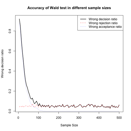
## [100,] 500 31 0 31 0.062plot(Wrong_Dec_matrix2[,1], Wrong_Dec_matrix2[,5], type = "l", lty=1, lwd=2, xlab = "Sample Size", ylab = "Wrong decision ratio", main = "Accuracy of Wald test in different sample sizes")
lines(Wrong_Dec_matrix2[,1], Wrong_Dec_matrix2[,2]/NREP, col="red",lty=2)
lines(Wrong_Dec_matrix2[,1], Wrong_Dec_matrix2[,3]/NREP, col="blue",lty=3)
legend("topright",c("Wrong decision ratio","Wrong rejection ratio","Wrong acceptance ratio"),lty=1:3,lwd=c(2,1,1),col = c("black","red","blue"))
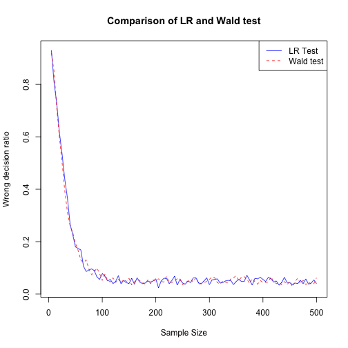
In the plot below, I compare LR and Wald test and we can see that there is no significant differnce between them in terms of convergence to best accuracy by sample size.
plot(Wrong_Dec_matrix[,1], Wrong_Dec_matrix[,5], type = "l", lty=1, col="blue", xlab = "Sample Size", ylab = "Wrong decision ratio", main = "Comparison of LR and Wald test")
lines(Wrong_Dec_matrix2[,1], Wrong_Dec_matrix2[,5], col="red",lty=2)
legend("topright", c("LR Test", "Wald test"), lty = c(1,2), col=c("blue","red"))