Change Point Analysis with a Bayesian Approach

In this post, I am going to perform a change-point analysis on coal-mining disasters time-series data from 1851 to 1962. For this analysis, we take a Bayesian approach and will see steps of Infering on this problem using Gibbs sampler (This is Exercise 7.6 from Computational statistics by G. H. Givens and J. A. Hoeting). Let us take a look at our data as the first step.

library(readr)
coal <- read_table2("/Users/hamed/Documents/Academics/Term 2/Applied Statistics I/Assignment4/datasets/coal.csv")

plot(coal$year, coal$disasters, type = 'l', xlab = "Year", ylab = "Disasters")

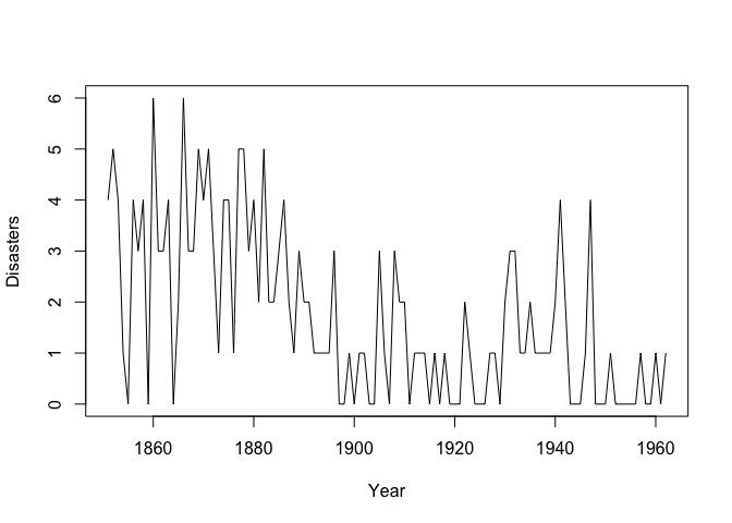
Visually, it can be noticed that there might be a change point in this time series data. For these data, we assume the hierarchical model:

\[X_j \sim \begin{cases} Poisson(\lambda_1) & j=1,..., \theta \\ Poisson(\lambda_2) & j=\theta +1,...,112 \end{cases}\]

Assume \(\lambda_i| \alpha \sim Gamma(3, \alpha)\) for i = 1, 2, where \(\alpha \sim Gamma(10, 10)\), and assume \(\theta\) follows a discrete uniform distribution over {1,…,111}. Now, we need to estimate the posterior distribution of the parameters using a Gibbs sampler. \(\theta\) is of a special interest for us since it is the change point we mean to estimate.

Deriving the conditional distributions

The target distribution is posterior distribution of parameters given data X:

\[p(\lambda_1, \lambda_2, \alpha, \theta |{\bf X}) = \frac{p(\lambda_1, \lambda_2, \alpha, \theta ,{\bf X})}{p({\bf X})}\]

To use Gibbs sampling approach, we need to derive conditional distribution of each of the parameters on the others:

\[p(\alpha|\lambda_1^{(t)}, \lambda_2^{(t)}, \theta^{(t)}, {\bf X}) \propto p(\lambda_1^{(t)}, \lambda_2^{(t)}, \theta^{(t)}, {\bf X}|\alpha) \times p(\alpha) \\= p(\lambda_1^{(t)}|\alpha)p(\lambda_2^{(t)}|\alpha)p({\bf X}, \theta^{(t)}|\lambda_1^{(t)},\lambda_2^{(t)})p(\alpha)\] \[= p(\lambda_1^{(t)}|\alpha)p(\lambda_2^{(t)}|\alpha)p(\theta^{(t)})p({\bf X}|\theta^{(t)},\lambda_1^{(t)},\lambda_2^{(t)})p(\alpha) \\ \propto p(\lambda_1^{(t)}|\alpha)p(\lambda_2^{(t)}|\alpha)p(\alpha)\]

Note that \(p(\theta^{(t)})\) and \(p({\bf X}|\theta^{(t)},\lambda_1^{(t)},\lambda_2^{(t)})\) in this equation are constants not dependent on \(\alpha\).

\[p(\lambda_1^{(t)}|\alpha)p(\lambda_2^{(t)}|\alpha)p(\alpha) = \frac{\alpha^3}{\Gamma(3)}\lambda_1^{(t)^2}e^{-\alpha \lambda_1^{(t)}} \times \frac{\alpha^3}{\Gamma(3)}\lambda_2^{(t)^2}e^{-\alpha \lambda_2^{(t)}} \times \frac{10^{10}}{\Gamma(10)}\alpha^9e^{-10\alpha}\]

Again, note that \(\lambda_1^{(t)^2}\) and \(\lambda_2^{(t)^2}\) are constants w.r.t \(\alpha\). So, we have:

\[\propto \alpha^{15} e^{-(\lambda_1^{(t)} +\lambda_2^{(t)} +10)\alpha} \propto Gamma(16, \lambda_1^{(t)^2} + \lambda_2^{(t)^2} + 10)\]

In a similiar way, it can be shown that:

\[p(\lambda_1^{(t)}|\lambda_2^{(t)}, \theta^{(t)},\alpha^{(t)}, {\bf X}) \propto Gamma(3+\sum_{i=1}^{\theta^{(t)}}x_i , \theta^{(t)}+\alpha^{(t)})\] \[p(\lambda_2^{(t)}|\lambda\_1^{(t)}, \theta^{(t)},\alpha^{(t)}, {\bf X}) \propto Gamma(3+\sum_{i=\theta^{(t)}+1}^{112}x_i, 112-\theta^{(t)}+\alpha^{(t)})\] \[p(\theta|\lambda_1^{(t)}, \lambda_2^{(t)},\alpha^{(t)} , {\bf X}) \propto \lambda_1^{\sum_{i=1}^{\theta}}\lambda_2^{\sum_{i=\theta+1}^{112}}e^{\theta(\lambda_1^{(t)} - \lambda_2^{(t)})}\]

Although it is not a known distribution, but we can easily sample from it in R using ‘sample’ function because \(\theta\)’s are discrete and the formula above is proportionate to pmf.

Implementing Gibbs sampler

Gibbs_sampler = function(lambda1=2, lambda2=2, alpha=3, theta=60, X, NREP=10000){
  n = length(X)
  theta_space = 1:(n-1)
  lambda1_ch = c(lambda1)
  lambda2_ch = c(lambda2)
  alpha_ch = c(alpha)
  theta_ch = c(theta)
  
  sum_to_theta = c()
  sum_from_theta = c()
  
  for (i in theta_space){
    sum_to_theta[i] = sum(X[1:i])
    sum_from_theta[i] = sum(X[(i+1):n])
  }
  
  for (i in 1:NREP){
    theta_pmf = (lambda1_ch[i] ^ sum_to_theta) * (lambda2_ch[i] ^ sum_from_theta) * exp(-theta_space * (lambda1_ch[i] - lambda2_ch[i]))   #This is not pmf, but pmf is proportionate to this
    theta_ch[i+1] = sample(theta_space, 1, prob=theta_pmf)
    
    lambda1_ch[i+1] = rgamma(1, sum(X[1:theta_ch[i+1]]) + 3, theta_ch[i+1] + alpha_ch[i])
    lambda2_ch[i+1] = rgamma(1, sum(X[(theta_ch[i+1]+1):n]) + 3, n - theta_ch[i+1] + alpha_ch[i])
    alpha_ch[i+1] = rgamma(1, 16, 10 + lambda1_ch[i+1] + lambda2_ch[i+1])
  }
  sample_mat = cbind(lambda1_ch, lambda2_ch, alpha_ch, theta_ch)
  colnames(sample_mat) = c("Lambda1", "Lambda2", "Alpha", "Theta")
  return(sample_mat)
}

X = coal$disasters
res = Gibbs_sampler(X=X)

NREP=10000
x = 1:(NREP+1)
par(mfrow=c(2,2))
plot(x, res[,1], type='l', ylab = "Lambda1", main = "Sample path of Lambda1")
plot(x, res[,2], type='l', ylab = "Lambda2", main = "Sample path of Lambda2")
plot(x, res[,3], type='l', ylab = "Alpha", main = "Sample path of alpha")
plot(x, res[,4], type='l', ylab = "Theta", main = "Sample path of theta")

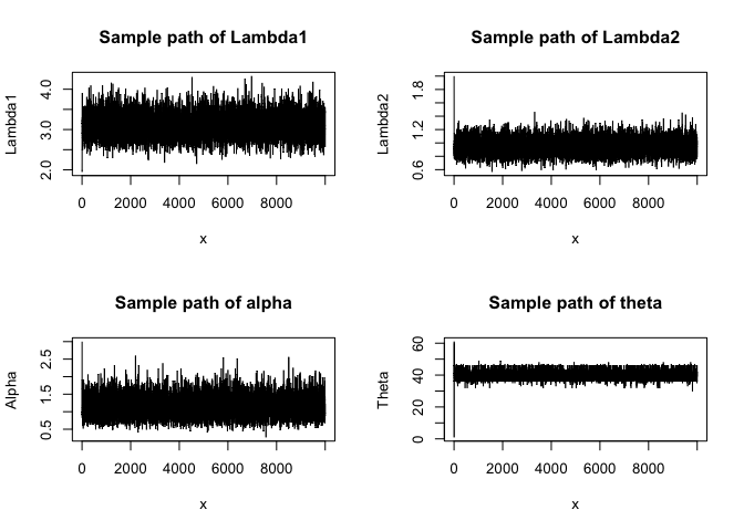
We can see that the samples are mixing and converging to the stationary distribution (i.e. the target distribution) of the chain. To verify this conclusion, we also employ ACF plots of these chains as diagnosis:

par(mfrow=c(2,2))
acf(res[,1], main = "Lambda1")
acf(res[,2], main = "Lambda2")
acf(res[,3], main = "Alpha")
acf(res[,4], main = "Theta")

ACF plots also confirms that the sample is convergent to the stationary distribution.

Density Histograms and Summary statistics

x = 1:(NREP+1)
par(mfrow=c(2,2))
hist(res[,1], xlab = "Lambda1", main = "Histogram of Lambda1", breaks = 50)
hist(res[,2], xlab = "Lambda2", main = "Histogram of Lambda2", breaks = 50)
hist(res[,3], xlab = "Alpha", main = "Histogram of alpha", breaks = 50)
hist(res[,4], xlab = "Theta", main = "Histogram of theta", breaks = 50)

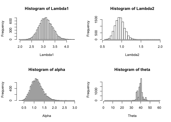
It does not seem that warming up is a serious issue for these chains, so I do not discard any realizations for estimation.

library(psych)
describe(res)

##         vars     n  mean   sd median trimmed  mad  min   max range  skew
## Lambda1    1 10001  3.11 0.29   3.10    3.10 0.29 1.95  4.33  2.37  0.18
## Lambda2    2 10001  0.95 0.12   0.95    0.95 0.12 0.57  2.00  1.43  0.29
## Alpha      3 10001  1.14 0.29   1.12    1.13 0.28 0.27  3.00  2.73  0.53
## Theta      4 10001 39.89 2.50  40.00   39.83 1.48 1.00 61.00 60.00 -0.07
##         kurtosis   se
## Lambda1     0.10 0.00
## Lambda2     0.71 0.00
## Alpha       0.54 0.00
## Theta       7.02 0.02

The important point is that since posterior distributions of parameters are not symmetric, conventinal CI’s will be misleading and it is better to use highest posterior density (HPD) to do inferences. The results of this model shows that up to 40th year the mean rate of incidents of accidents are 3.11 and after this change point the mean rate decreases to 0.95.