Finite difference method for pricing european options

When pricing options with Black-Scholes equations, among the Finite-Difference methods to solve the equation, Crank-Nicolson method is the most accurate and always numerically stable. In this post, After a brief explanation of the method, its Python implementation is presented.

Crank-Nicolson method is the average of implicit and explicit (FDM) approximation of Black-Scholes equation. Meaning that the approximated equation is derived from averaging two sides of implicit and explicit approximation. Therefore we have:

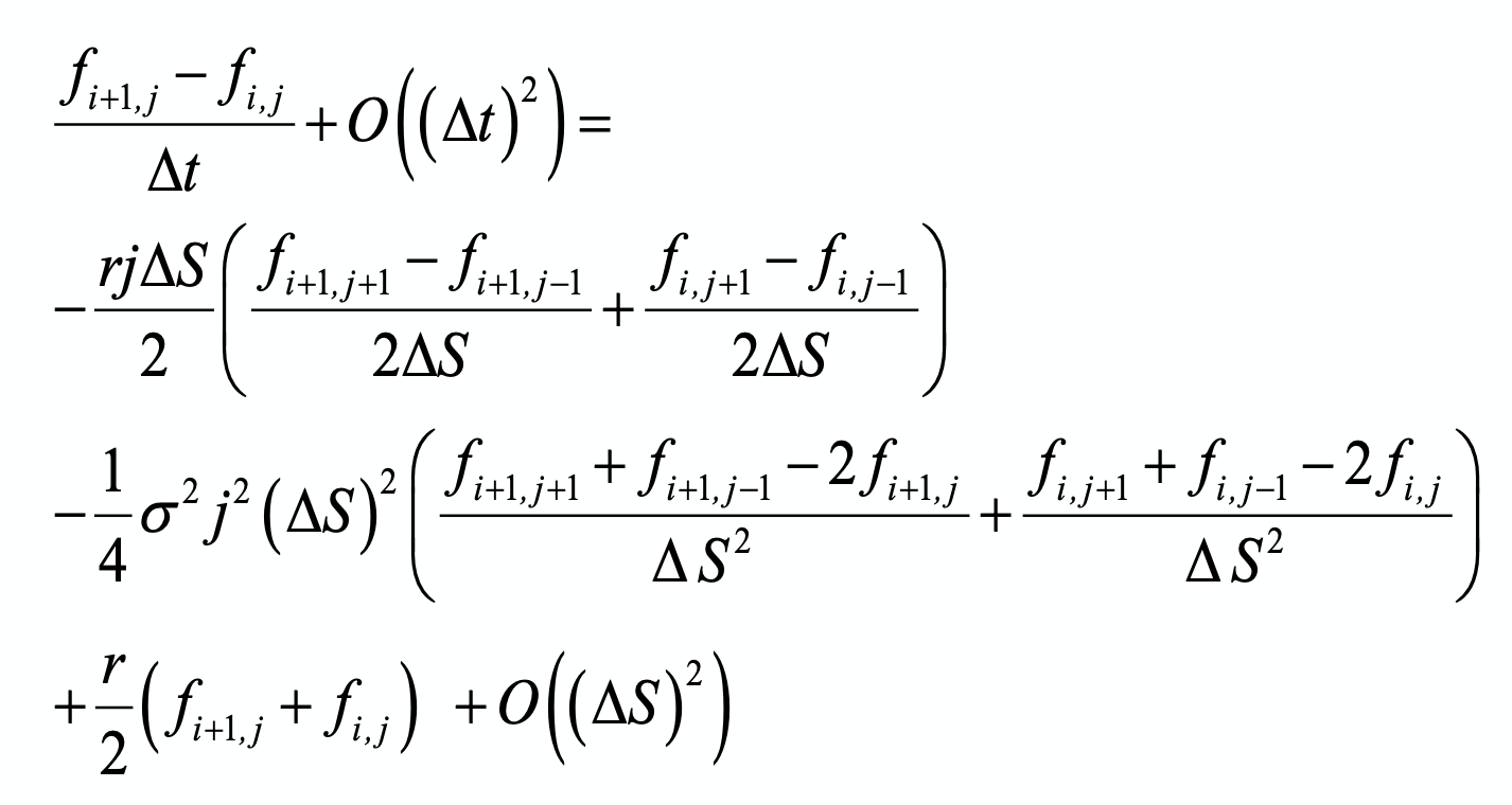
Note that remaining terms (say the error term of approximation) is from the second order of \(\delta t\). Rewriting the equation, we can get Crank-Nicolson scheme:

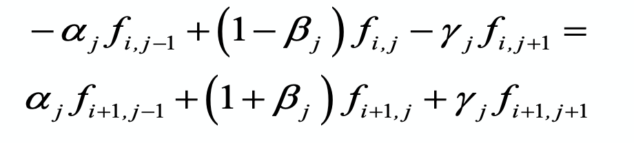
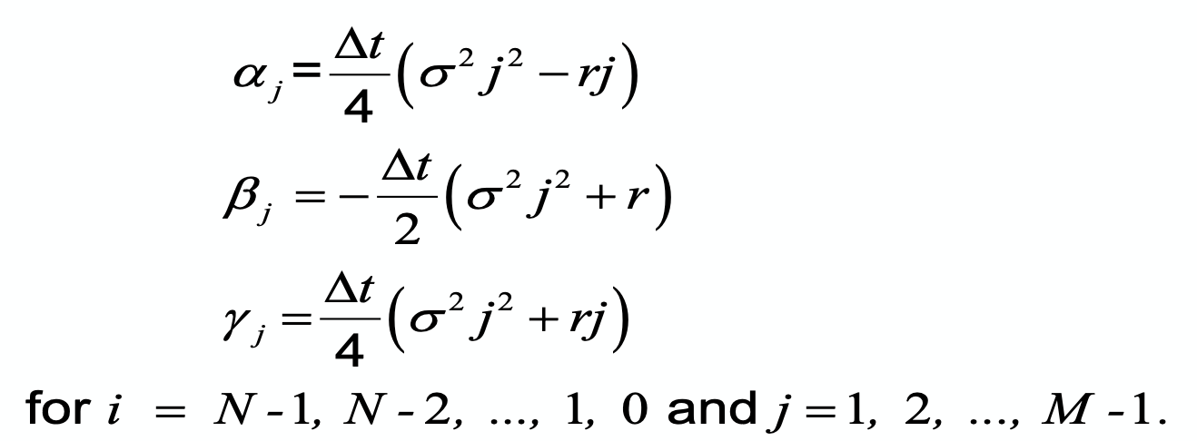
Where:

Implementation Notes

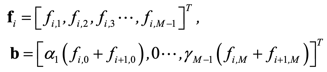
The scheme equation can be rewritten in matrix form:

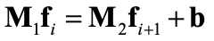
Where \(f_i\) and \(b_i\) are (M-1) dimensional vectors:

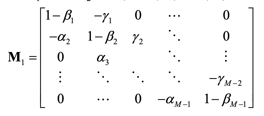
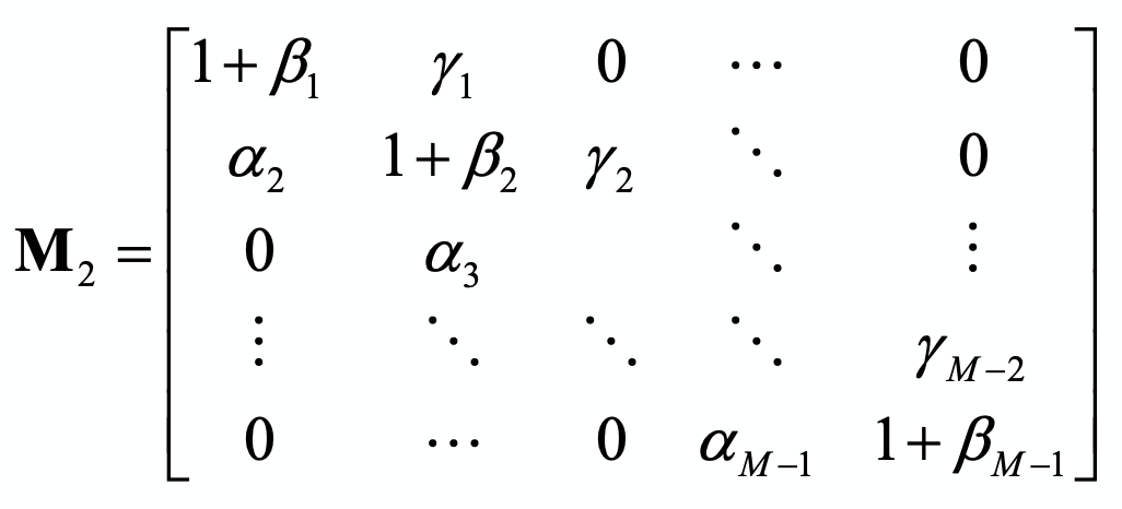
And \(M_1\) and \(M_2\) are \((M-1) \times (M-1)\) symmetric matrices:

Implementation in Python

Suppose we aim to price a european put option with features as follows:

T = 6/12 #period of contract
S_0 = 30  #price at time zero
K = 34  #exercise price
sigma = 0.3  #Volatility
r = 0.1  #Risk-neutral interest-rate
price = 0  #Just initialization :)

import numpy as np

S_max = 80

N = 500
M = 50
dt = T / N
ds = S_max / M

f = np.zeros((M+1,N+1))  # The array f is the mesh of approximation of the option price function
I = np.arange(0, M+1)
J = np.arange(0, N+1)

# Boundary and final conditions
f[:, N] = np.maximum(K - (I * ds), 0)
f[0, :] = K * np.exp(-r * (T - J * dt))
f[M, :] = 0

alpha = 0.25 * dt * (sigma**2 * (I**2) - r * I)
beta = -dt * 0.5 * (sigma**2 * (I**2) + r)
gamma = 0.25 * dt * (sigma**2 * (I**2) + r * I)

M1 = np.diag(1-beta[1:M]) + np.diag(-alpha[2:M], k=-1) + np.diag(-gamma[1:M-1], k=1)
M2 = np.diag(1+beta[1:M]) + np.diag(alpha[2:M], k=-1) + np.diag(gamma[1:M-1], k=1)

for j in range(N-1, -1, -1):
    l = np.zeros(M - 1)
    l[0] = alpha[1] * (f[0, j] + f[0, j+1])
    l[-1] = gamma[M-1] * (f[M, j] + f[M, j+1])
    f[1:M, j] = np.linalg.solve(M1, M2 @ f[1:M, j+1] + l)

## Finding the price by interapolation
idown = int(np.floor(S_0 / ds))
iup = int(np.ceil(S_0 / ds))
print(idown)
print(iup)
if idown == iup:
    price = f[idown, 0]
else:
    price = f[idown, 0] + ((iup - (S_0 / ds)) / (iup - idown)) * (f[iup, 0] - f[idown, 0])

print(price)

18
19
4.476727373720464

A trick to simpler implementation

If you do the transformation \(Z=ln(S)\) and take the similar path of extracting equation and scheme, you can easily see that all \(\alpha_i\)s are equal and the same is for \(\beta_i\)s and \(\gamma_i\)s. Then the implentation code will be:

Z_0 = np.log(S_0)
Z_max = np.log(S_max)

dz = Z_max / M

f = np.zeros((M+1,N+1))
I = np.arange(0, M+1)
J = np.arange(0, N+1)

# Boundary and final conditions
f[:, N] = np.maximum(K - np.exp(I * dz), 0)
f[0, :] = K * np.exp(-r * (T - J * dt))
f[M, :] = 0

a = sigma**2/(4*dz**2) - (r-sigma**2/2)/(4*dz)
b1 = - (1/dt + 0.5*r + sigma**2/(2*dz**2))
b2 = -1/dt + 0.5*r + sigma**2/(2*dz**2)
c = sigma**2/(4*dz**2) + (r-sigma**2/2)/(4*dz)

# Solving for f
M1 = b1 * np.eye(M-1) + a * np.eye(M-1, k=-1) + c * np.eye(M-1, k=1)
M2 = b2 * np.eye(M-1) - a * np.eye(M-1, k=-1) - c * np.eye(M-1, k=1)

for j in range(N-1, -1, -1):
    l = np.zeros(M - 1)
    l[0] = - a * (f[0, j] + f[0, j+1])
    l[-1] = - c * (f[M, j] + f[M, j+1])
    f[1:M, j] = np.linalg.solve(M1, M2 @ f[1:M, j+1] + l)

# finding the price
idown = int(np.floor(Z_0 / dz))
iup = int(np.ceil(Z_0 / dz))
print(idown)
print(iup)
if idown == iup:
    price = f[idown, 0]
else:
    price = f[idown, 0] + ((iup - (Z_0 / dz)) / (iup - idown)) * (f[iup, 0] - f[idown, 0])

print(price)

38
39
5.007811432429777